Statistical power is the probability that a specified test will reject its null hypothesis when a particular alternative is true. In a cannabis plant study, it describes how often the planned analysis would detect a defined difference under stated assumptions. It isn’t the probability that your hypothesis is right, and it isn’t a guarantee that a study will find something useful.
The null hypothesis is the reference claim the test evaluates, often no mean difference. The alternative specifies the difference the design should be able to detect. Missing that real difference is a false negative; power is one minus the probability of that error for the specified alternative.
Choose the difference before counting samples
The first design question is what difference would change your interpretation. A study intended to detect a large difference in an ordinary plant trait can need a different design from one intended to distinguish very similar groups. If you skip that question and ask only how many plants you need, there’s no single defensible answer.
Write the outcome, its units, the comparison and the smallest effect size worth detecting before looking for a sample-size calculator. Then identify the independent replication available for that comparison. The site’s explanation of experimental units in clone trials is important here: extra leaves or repeated instrument readings can improve measurement, but they don’t create new independent treatment assignments.
Power depends on the specified effect, variability, sample size, significance threshold and analysis. NIST explains why sample-size planning needs those assumptions. They’re general statistical principles; they don’t establish a universal sample count for cannabis.
Make the assumptions visible in a sensitivity table
Before commissioning a calculation, prepare a small table with one row per plausible scenario. Include the meaningful difference, expected variability, available independent units and anticipated missing observations. For each row, ask for power under the intended model or the sample size needed for a chosen power target.
Use a pilot or comparable research to justify variability, while acknowledging that a small pilot can estimate it poorly. Include a less favorable scenario rather than selecting the single assumption that makes your budget look adequate. The purpose is to see how fragile the plan is, not to obtain a reassuring percentage.
A worked planning example
For illustration only, compare two independent, equally sized groups with normally distributed measurements, a common standard deviation and a two-sided 0.05 test. Using 80% power as an example target, a normal approximation gives n per group = 2 x (1.95996 + 0.84162)2 x (SD / difference)2. The two normal-distribution quantiles are approximately 1.96 and 0.84; the calculation retains extra digits. ICAR-NIVEDI gives the two-independent-means planning formula.
| Difference (mm) | Common SD (mm) | Approximate n per group |
|---|---|---|
| 2 | 4 | 63 |
| 4 | 4 | 16 |
| 2 | 8 | 252 |
These are invented assumptions, rounded up, with no allowance for losses or clustering. They’re not recommended cannabis sample sizes; a t-test calculation with estimated variance can differ. The lesson is the sensitivity: halving the target difference or doubling the SD roughly quadruples the required independent units. If your budget only supports detection of large differences, change the design or narrow the promise before collecting data.
Match the calculation to the real comparison
The experimental design matters: paired measurements, clustered units and repeated observations require their own assumptions. A calculation for two unrelated groups may be inappropriate when the same units are measured twice or many samples share one experimental setting. For a comparison spanning environments, genotype-by-environment interaction also explains why you may need to estimate more than one average difference.
Ask how the proposed analysis handles those relationships and whether the calculation includes them. If several outcomes or many markers will be tested, the error-control plan can change the detection threshold as well. A simple calculator cannot decide those design questions for you.
A conventional target such as 80% power is a planning choice. Whether it’s adequate depends on the consequences of missing an effect, the available resources and the strength of evidence needed. Increasing the false-positive threshold just to make the power figure rise changes the error tradeoff; it doesn’t improve the experiment for free.
Read a completed study differently
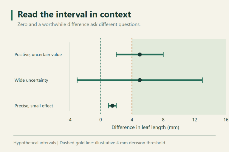
After the data exist, inspect the estimated effect and its uncertainty rather than calculating “observed power” from that same effect and treating it as new evidence. Hoenig and Heisey explain the problem with that post-hoc calculation. A nonsignificant result may be compatible with both a negligible difference and a practically important one. The interval and design tell you which conclusions remain plausible.
A useful study report states what it was designed to detect, the assumptions behind that plan, the independent units actually analyzed and any losses or deviations. If the analysis is clustered, involves several traits or will support a costly decision, involve a statistician before data collection. That lets the design change while change can still help.